
Let’s consider elliptic problem (*) on the square 0≤x≤1, 0≤y≤1 with Laplace operator

On the sides of the square we set boundary conditions
u(0, y) = u(1, y) = u(x, 0) = u(x, 1) = 0, 0≤x≤1, 0≤y≤1.
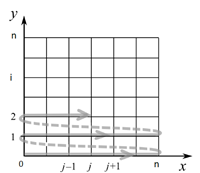
To prepare the grid we subdivide the square on n2 equal small squares and apply finite differences schema both on axis x and on axis y with h = 1/n.
This way we get a vector of unknowns u indexed by two indexes i = 0, …, n and j = 0, …, n (because we did discretization by two variables x and y).
In order to get more convenient indexing with one index, we reorder coordinates of vector u lexicographically (first we get all coordinates with i = 0, then all coordinates with i = 1, and so on).
As a result, we receive a block-diagonal matrix of the form:
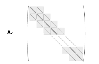
This matrix has dimensions N х N, where N = (n + 1)2.
On its main diagonal, it has 3-diagonal blocks (of the size n + 1) quite similar to matrix А1 from the 1-dimensional problem – we just need to replace all numbers 2 in this matrix to numbers 4 (i.e. the diagonal should contain numbers 4 + σj instead of 2 + σj, j = 0, …, n).
The blocks upper and below blocks of the main diagonal are diagonal matrices of the size n + 1 with -1 on the main diagonal
Thus, 2-dimensional problem becomes a little bit more complicated, but not too much. The matrix is still very sparse. Moreover, it is symmetric and even positive defined. This allows to solve this problem very efficiently using, for instance, conjugate gradients method.